Spatial Lag Model
Introduction
The Spatial Lag Model (SLM) is a fundamental concept in the field of spatial econometrics. It is a statistical model that incorporates spatial dependence into regression analysis. The SLM is used to model situations where the value of an observation is influenced by the values of neighboring observations.


Concept and Definition
The Spatial Lag Model is based on the principle of spatial autocorrelation, which asserts that data points located close to each other in space are more likely to have similar values than those that are further apart. This principle is encapsulated in Tobler's First Law of Geography: "Everything is related to everything else, but near things are more related than distant things."
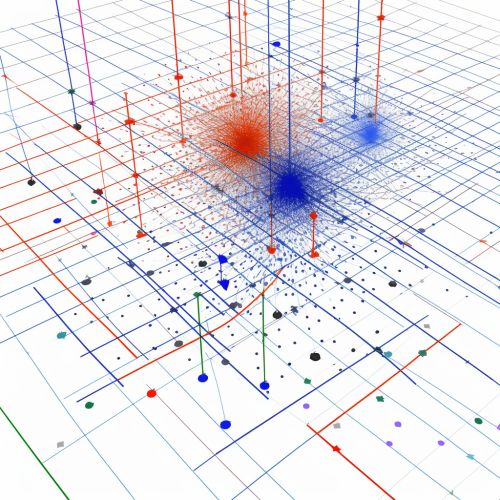
In the SLM, the dependent variable in a regression model is influenced not only by the independent variables, but also by the values of the dependent variable at neighboring locations. This influence is represented by a spatial weights matrix, which defines the relationships between different locations.
Mathematical Formulation
The Spatial Lag Model can be mathematically represented as follows:
Y = ρWY + Xβ + ε
Here, Y is the dependent variable, X is a matrix of independent variables, β is a vector of coefficients, ε is the error term, W is the spatial weights matrix, and ρ is the spatial autoregressive parameter.
The spatial weights matrix W is a square matrix that defines the spatial relationships between observations. Each element of W represents the influence of one observation on another. The spatial autoregressive parameter ρ measures the strength of the spatial dependence.
Estimation and Interpretation
Estimating the parameters of a Spatial Lag Model typically involves the use of maximum likelihood estimation. This method finds the values of ρ and β that maximize the likelihood of the observed data given the model.
Interpreting the results of a Spatial Lag Model can be more complex than interpreting a standard regression model. The coefficient β represents the direct effect of the independent variables on the dependent variable. However, the spatial autoregressive parameter ρ represents the indirect effect of the dependent variable at neighboring locations on the dependent variable at a given location.
Applications
The Spatial Lag Model has wide-ranging applications in various fields such as economics, geography, sociology, and environmental science. It is particularly useful in situations where spatial dependence is expected to play a significant role. For example, it can be used to model the spread of diseases, the diffusion of innovations, or the spatial distribution of economic activity.
Limitations and Extensions
While the Spatial Lag Model is a powerful tool for modeling spatial dependence, it also has some limitations. One major limitation is the assumption of stationarity, which means that the spatial relationships are assumed to be constant over space. In reality, these relationships may vary across different locations.
To address this limitation, several extensions of the Spatial Lag Model have been proposed. These include the Geographically Weighted Regression (GWR) model, which allows the spatial relationships to vary over space, and the Spatial Durbin Model (SDM), which incorporates both spatial lag and spatial error dependence.
