Discrete Uniform Distribution

Introduction

The discrete uniform distribution is a type of probability distribution in which a finite number of outcomes are equally likely to occur. This distribution is a fundamental concept in probability theory and statistics, often used in scenarios where each outcome of a finite set is equally probable.

Definition

A discrete uniform distribution is defined over a finite set of integers. If the set of possible outcomes is \(\{a, a+1, a+2, \ldots, b\}\), where \(a\) and \(b\) are integers and \(a \leq b\), then the probability mass function (PMF) is given by:

\[ P(X = k) = \frac{1}{b - a + 1} \]

for \(k = a, a+1, \ldots, b\).

Properties

Mean

The mean (or expected value) of a discrete uniform distribution is the average of the smallest and largest values in the set:

\[ \mu = \frac{a + b}{2} \]

Variance

The variance of a discrete uniform distribution measures the spread of the values around the mean:

\[ \sigma^2 = \frac{(b - a + 1)^2 - 1}{12} \]

Moment Generating Function

The moment generating function (MGF) of a discrete uniform distribution is used to derive moments of the distribution. It is given by:

\[ M_X(t) = \frac{e^{at} - e^{(b+1)t}}{(b - a + 1)(1 - e^t)} \]

for \(t \neq 0\).

Applications

Discrete uniform distributions are widely used in various fields such as computer science, engineering, and finance. Some common applications include:

**Random Number Generation**: Discrete uniform distributions are often used in algorithms for generating random numbers.
**Simulations**: In Monte Carlo simulations, discrete uniform distributions are used to model random events with equally likely outcomes.
**Games of Chance**: Many games, such as rolling a fair die or drawing a card from a well-shuffled deck, are modeled using discrete uniform distributions.

Examples

Rolling a Die

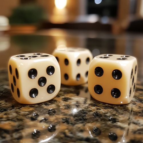
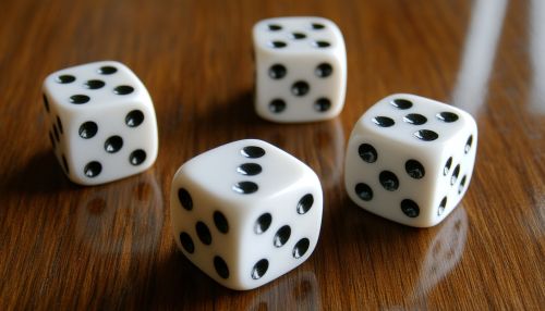
A classic example of a discrete uniform distribution is the roll of a fair six-sided die. The possible outcomes are \(\{1, 2, 3, 4, 5, 6\}\), and each outcome has a probability of \(\frac{1}{6}\).

Drawing a Card

Another example is drawing a card from a standard deck of 52 cards. If we are interested in the rank of the card, the possible outcomes are \(\{1, 2, \ldots, 13\}\), each with a probability of \(\frac{1}{13}\).

Relationship with Other Distributions

The discrete uniform distribution is closely related to other probability distributions:

**Continuous Uniform Distribution**: The continuous counterpart of the discrete uniform distribution, defined over a continuous interval \([a, b]\).
**Binomial Distribution**: When considering the number of successes in a series of independent Bernoulli trials, the binomial distribution can be seen as a generalization of the discrete uniform distribution.

Estimation and Testing

Parameter Estimation

The parameters \(a\) and \(b\) of a discrete uniform distribution can be estimated using the method of moments or maximum likelihood estimation (MLE). For a sample \(X_1, X_2, \ldots, X_n\), the MLEs are:

\[ \hat{a} = \min(X_i) \] \[ \hat{b} = \max(X_i) \]

Hypothesis Testing

To test whether a given sample follows a discrete uniform distribution, statistical tests such as the chi-square goodness-of-fit test can be used.

Limitations

While the discrete uniform distribution is useful in many scenarios, it has limitations. It assumes that all outcomes are equally likely, which may not be realistic in all situations. Additionally, it is only applicable to finite sets of outcomes.

References

Feller, W. (1968). An Introduction to Probability Theory and Its Applications. Vol. 1. Wiley.
Ross, S. M. (2014). Introduction to Probability Models. Academic Press.
Grimmett, G., & Stirzaker, D. (2001). Probability and Random Processes. Oxford University Press.