Beta distribution: Difference between revisions
(Created page with "== Introduction == The '''Beta distribution''' is a family of continuous probability distributions defined on the interval [0, 1], parameterized by two positive shape parameters, denoted by α (alpha) and β (beta). It is widely used in various fields such as Bayesian statistics, order statistics, and reliability engineering due to its flexibility in modeling random variables that are constrained within a finite interval. == Definition and Properties == The probabilit...") |
No edit summary |
||
| Line 91: | Line 91: | ||
== References == | == References == | ||
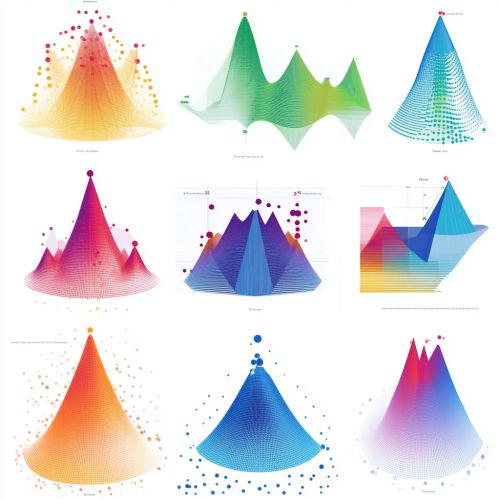
[[Image:Detail-97567.jpg|thumb|center|Graphical representation of Beta distribution with different shape parameters.|class=only_on_mobile]] | |||
[[Image:Detail-97568.jpg|thumb|center|Graphical representation of Beta distribution with different shape parameters.|class=only_on_desktop]] | |||
[[Category:Probability distributions]] | [[Category:Probability distributions]] | ||
[[Category:Bayesian statistics]] | [[Category:Bayesian statistics]] | ||
[[Category:Reliability engineering]] | [[Category:Reliability engineering]] | ||
Latest revision as of 08:12, 11 August 2024
Introduction
The Beta distribution is a family of continuous probability distributions defined on the interval [0, 1], parameterized by two positive shape parameters, denoted by α (alpha) and β (beta). It is widely used in various fields such as Bayesian statistics, order statistics, and reliability engineering due to its flexibility in modeling random variables that are constrained within a finite interval.
Definition and Properties
The probability density function (PDF) of the Beta distribution is given by:
\[ f(x; \alpha, \beta) = \frac{x^{\alpha-1} (1-x)^{\beta-1}}{B(\alpha, \beta)} \]
where \( B(\alpha, \beta) \) is the Beta function, defined as:
\[ B(\alpha, \beta) = \int_0^1 t^{\alpha-1} (1-t)^{\beta-1} \, dt \]
The Beta function serves as a normalization constant to ensure that the total probability integrates to 1. The parameters α and β shape the distribution, allowing it to take various forms such as uniform, U-shaped, or J-shaped distributions.
Moments and Statistics
The moments of the Beta distribution can be derived from its PDF. The mean (expected value) and variance are given by:
\[ \text{Mean} = \frac{\alpha}{\alpha + \beta} \]
\[ \text{Variance} = \frac{\alpha \beta}{(\alpha + \beta)^2 (\alpha + \beta + 1)} \]
Higher-order moments, such as skewness and kurtosis, provide additional insights into the distribution's shape. Skewness is given by:
\[ \text{Skewness} = \frac{2(\beta - \alpha) \sqrt{\alpha + \beta + 1}}{(\alpha + \beta + 2) \sqrt{\alpha \beta}} \]
Kurtosis is given by:
\[ \text{Kurtosis} = \frac{6[(\alpha - \beta)^2 (\alpha + \beta + 1) - \alpha \beta (\alpha + \beta + 2)]}{\alpha \beta (\alpha + \beta + 2) (\alpha + \beta + 3)} \]
Parameter Estimation
Parameter estimation for the Beta distribution can be performed using methods such as the method of moments or maximum likelihood estimation (MLE). Given a sample of data, the method of moments involves equating the sample moments to the theoretical moments and solving for the parameters α and β.
In MLE, the log-likelihood function is maximized with respect to the parameters. The log-likelihood function for a sample \( x_1, x_2, \ldots, x_n \) is:
\[ \log L(\alpha, \beta) = (\alpha - 1) \sum_{i=1}^n \log x_i + (\beta - 1) \sum_{i=1}^n \log (1 - x_i) - n \log B(\alpha, \beta) \]
Solving the resulting equations typically requires numerical methods due to the complexity of the Beta function.
Applications
The Beta distribution is extensively used in various domains:
Bayesian Statistics
In Bayesian statistics, the Beta distribution serves as a conjugate prior for the Bernoulli, binomial, negative binomial, and geometric distributions. This means that if the prior distribution of a probability parameter is Beta-distributed, the posterior distribution will also be Beta-distributed after observing data.
Order Statistics
In order statistics, the Beta distribution describes the distribution of the k-th order statistic from a uniform (0, 1) sample. Specifically, the k-th order statistic follows a Beta distribution with parameters k and n-k+1, where n is the sample size.
Reliability Engineering
In reliability engineering, the Beta distribution is used to model the distribution of reliability metrics such as the probability of success or failure of a system component over a specified interval.
Relationship to Other Distributions
The Beta distribution is related to several other distributions:
- The Beta distribution is a special case of the Dirichlet distribution when the number of parameters is two. - When α = β = 1, the Beta distribution reduces to the uniform distribution on [0, 1]. - The Beta distribution is a generalization of the uniform distribution, allowing for more flexible modeling of probabilities.
Generalizations
The Beta distribution can be generalized in several ways:
Beta Prime Distribution
The Beta prime distribution is a related distribution defined on the positive real line. It is used in Bayesian inference as a conjugate prior for the precision of a normal distribution.
Generalized Beta Distribution
The generalized Beta distribution extends the Beta distribution to allow for different ranges other than [0, 1]. This generalization is useful in modeling data that is constrained within arbitrary finite intervals.
Computational Methods
Computing probabilities and quantiles for the Beta distribution often involves numerical techniques. Standard statistical software packages provide functions for evaluating the PDF, cumulative distribution function (CDF), and quantiles of the Beta distribution.
See Also
References


